Introduction
The electromagnetic (EM) signals measured from our drones are affected by many factors including the orientation, position and altitude of the magnetic sensor, the location and shape of the transmitter coil on the ground, the frequency content of the measured signal and most importantly the electromagnetic properties of the subsurface (mainly the electric resistivity).
How can we turn the signal measured with our drone EM system into information of these electric properties of the subsurface?
The process that is required for this is called an inversion. In DroneSOM project we have developed a new 3D inversion software capable of turning the measured drone EM data into a 3-dimensional model of the subsurface. This mathematically non-linear, non-unique and ill-posed problem requires extensive computational resources. Typically, one inversion run can easily take multiple days on a high-performance computing cluster consuming hundreds of GBytes of memory.
3D inversion
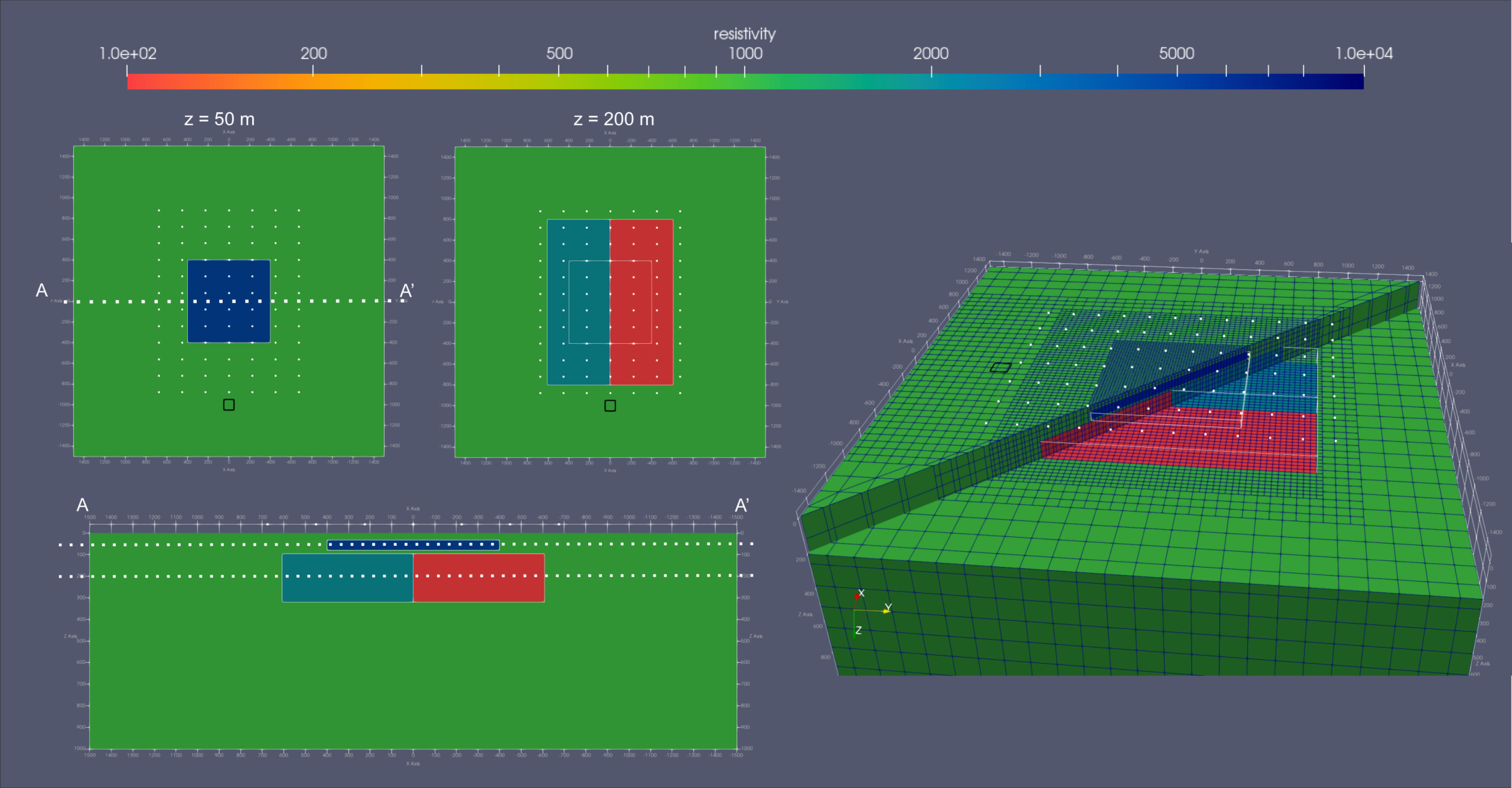
Here I will describe the general workflow and main concepts of our inversion procedure. The relationship between electric resistivity and the measured signal is governed by a set of partial differential equations (PDEs). Solving these PDEs for a given resistivity distribution allows us to compute the synthetic response that we would expect to measure for the given resistivity model, which is usually referred to as the forward problem. Figure 1 shows a simple benchmark model that we used to test our inversion against. To solve the forward problem, we use the finite element method. An octree grid (see the right 3D view in Fig 1) allows us to locally refine the grid where higher resolution is required while keeping the additional computational costs manageable. Each grid cell is assigned its own unique resistivity value.

Figure 1 Benchmark resistivity model used to verify the correctness of our new 3D inversion. The model consists of 3 boxes of different resistivities (100, 2 000 and 10 000 Ωm) embedded in a homogeneous background. There is 100 x 100 m loop source at the surface marked as black line and 84 drone soundings in 40 m height marked by white dots. On the left slices through the resistivity model in horizontal direction (upper panel) at 50 and 200m depth and vertical direction along profile AA’ in the lower panel. On the right, 3D view of the model also highlighting the Octree-mesh.
The inversion than describes the process of finding a resistivity distribution of the subsurface that when solving the forward problem matches with our measured data. This requires iteratively solving the forward problem until a resistivity model of the subsurface is found that explains the measured data sufficiently well. To do that we employ a flatness constrained Gauss-Newton optimization scheme. Meaning we look for a model that explains our measured data while also keeping the contrasts between neighbouring cells small resulting in a smooth looking image. The code has been written in C++ using the Deal.II library for all the finite element computations, PETSc for the linear algebra in the inversion and is parallelised across many CPUs using MPI.
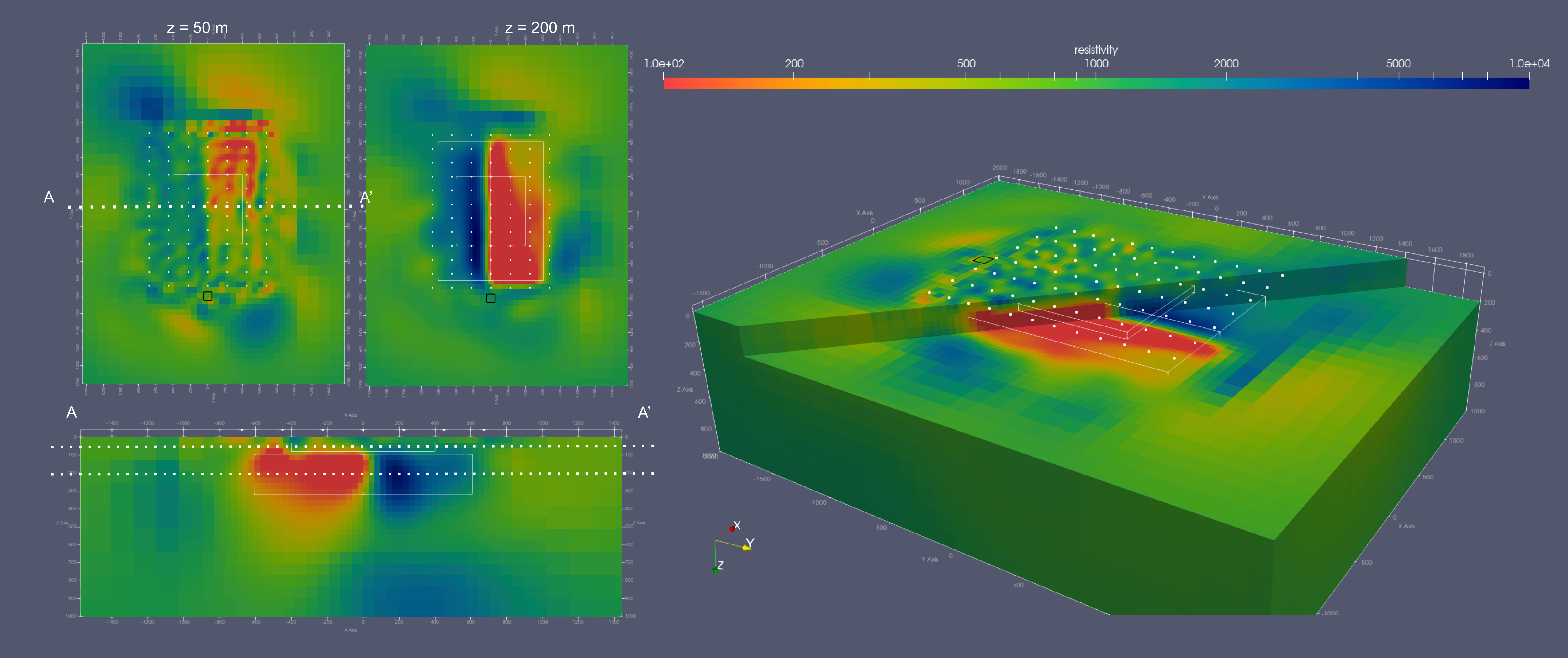
An example of an inversion of the synthetic benchmark model is shown in Fig. 2. Clearly the top and width of the conductive box is well recovered. At large distances to the transmitter loop the depth of conductive box is not well resolved and it appears to be closer to surface. Presence of the resistive box at depth is clearly visible although its outlines are not as well refined. The highly resistive and shallow anomaly however is not visible.

Figure 2 3D inversion image of the benchmark resistivity model shown in Fig. 1. There is 100 x 100 m loop source at the surface marked as black line and 84 drone soundings in 40 m height marked by white dots. For comparison, the location of the anomalous boxes is highlighted as thin white lines. On the left slices through the resistivity model in horizontal direction (upper panel) at 50 and 200m depth and vertical direction along profile AA’ in the lower panel. On the right, 3D view of the model.
In addition of testing the functionality of our inversions these synthetic tests are also a highly valuable tool for the actual survey design. Optimizing the survey parameters, such as source receiver layout, frequency content, etc., using a conceptual model of the expected target are crucial in ensuring a good resolution of the target structure. E.g. this small-scale example shows that electrically conductive targets are generally better resolved using a horizontal loop source. To ensure good resolution to resistive targets a grounded electric dipole source is the preferred type of source. Also, the depth of the conductive anomaly is not well resolved at large offsets to the transmitter loop. Thus, a repeating the survey if a second loop source will ensure adequate resolution everywhere in the model.
As shown our new 3D inversion algorithm is now running and has been tested on various synthetic test cases as well ground based field data and will be applied to the first real world drone data in autumn this year.
Authors
Cedric Patzer
Senior Scientist
Geological Survey of Finland
&
Longying Xiao
Senior Scientist
Geological Survey of Finland
